You can show numbers in thousands in Excel as K by using format code or additional calculations. It makes it easier to read large numbers in a table or chart. In the same way, you can display numbers in millions in Excel as M. If you can use calculations, you can divide numbers by 1000 to get results in thousands, but the usage of format code is a little bit complicated. Meanwhile, the original data is not changed.
Know your thousand separator settings in Excel
You can use excel format code to show numbers in thousands (K) or millions (M) in Excel, but first, you have to check which symbol it is using to group digits.
First of all, look into the Excel options. In my case, it is a comma. It is important because, in your situation, it might be a dot or space.
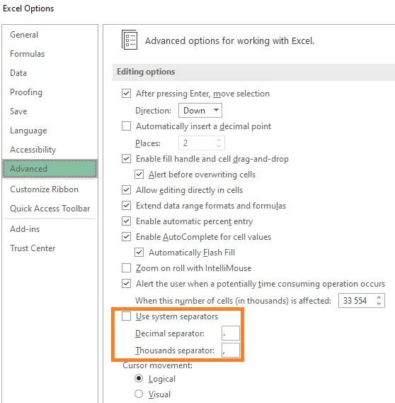
If there is a checkmark in Excel options that you are using system separators, look at the Region settings in the Control Panel.
Show numbers in thousands (K) in the Excel table
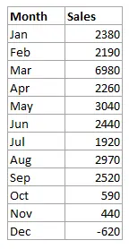
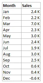
I have a table like this.
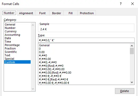
The easiest way to show numbers in thousands is to select numbers, open the Format Cells window (Ctrl + 1), and use a format code in the Custom section. In this case, hashtags ensure that numbers in millions will have a thousand separator, but in this table, it is not necessary.
#,##0.0," K"
Here is the result.
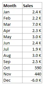
If you don’t want to see decimal places, you can use format code like this. But be careful if there is something below a thousand.
#,##0," K"
Look at this post if you want to learn more about format code in Excel.
Show numbers in millions (M) in the Excel table
If you want to display numbers in millions in Excel, use two thousand separators like this.
#,##0.0,," M"
Show numbers in thousands in Excel table conditionally
By using format code in Excel, you can create conditions. For example, if you want to show numbers in thousands with K above 1000 and below -1000, you can use this code.
[>=1000]#,##0.0," K";[<=-1000]-#,##0.0," K";0
Be careful with this approach, because it might be harder to read if you have to switch between units.
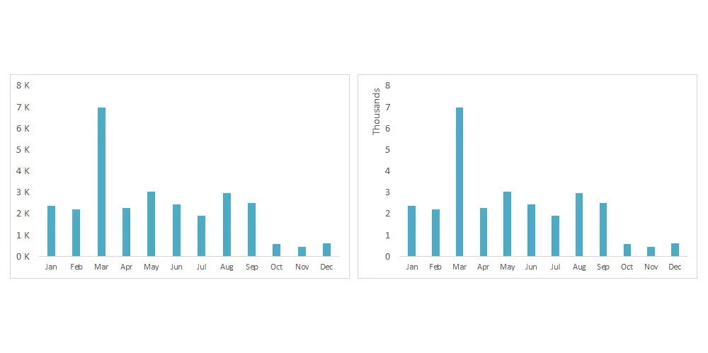
Show in thousands (K) or millions (M) on the Excel chart axis
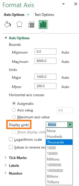
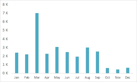
If you want to show numbers in thousands or millions on the Excel chart axis, change the axis display units options.
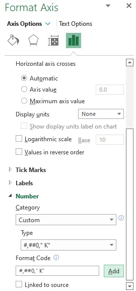
Format axis (select axis labels, and press Ctrl + 1) and change display units like this.
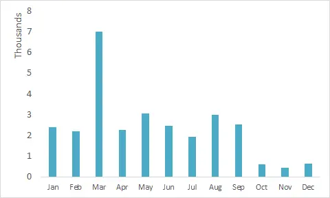
As the result, you will get something like this.
If it is not what you want, you can use format code to show numbers in thousands on the chart Y axis. After using the format code in the chart source table, the chart will automatically use that in the axis and data labels. In the situation when you can not use format code in the source table, use format code in the axis number formatting section.
#,##0," K"
That zero behind a hash symbol is important to display zero on the axis.
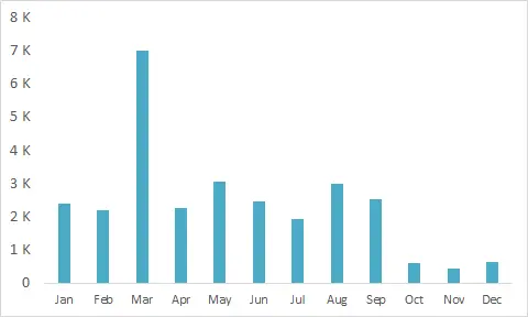
If you want to display zero without K or as empty space, you can separately format positive, negative, and zero values like this.
#,##0," K";-#,##0," K";0
Here is another example that uses format code to create conditional formatting for vertical or horizontal Excel chart axis.
Take a look at other Excel data visualizations in this blog: magic quadrant chart, gradient line chart, Pac man chart, glowing line chart, stripchart, and others.
Leave a Reply