
It is a good idea to add conditional formatting to Excel PivotTable. PivotTable is a great tool to create flexible data summaries and conditional formatting. Flexible approach to get necessary accents. Here are 3 easy steps to add conditional formatting to Excel PivotTable and a few things to keep in mind.
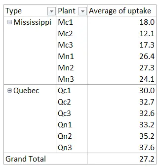
Here is my Excel PivotTable without conditional formatting. To build that, I used the CO2 dataset by using R.

By the way, if you are an experienced Excel user and want to know how to get your hands on R, I recommend you this post.
Add conditional formatting to Excel PivotTable
Follow these 3 easy steps on how to add conditional formatting to PivotTable. This approach will be flexible for variable rows and columns.
1. Select any calculated cell in PivotTable.
2. Go to the Conditional Formatting tool in the Excel Home tab and choose one of the options.
3. Look at the right side of the previously selected PivotTable cell. You will see a little icon.
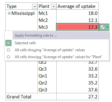

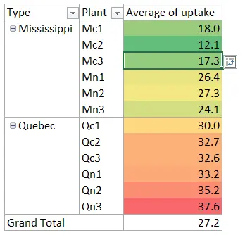
Choose how to apply conditional formatting. If you don’t know which option is the best, you can switch to the necessary one through the same icon.

Be careful. Additional PivotTable grouping level might be the reason why conditional formatting in PivotTable disappears.
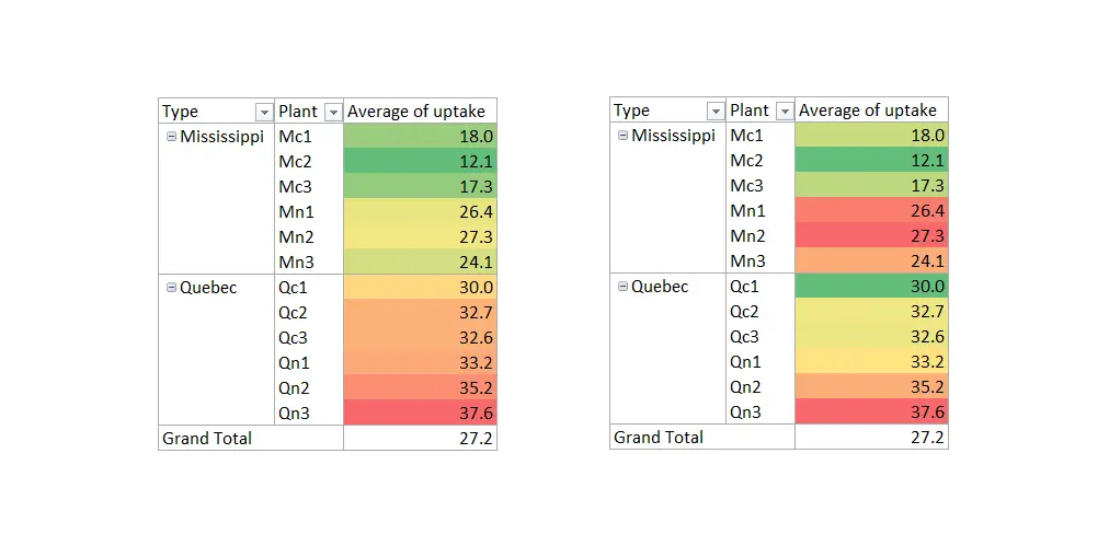
Independent conditional formatting for each Excel PivotTable group
If you want your conditional formatting for each group independently, you can do that by selecting necessary ranges separately.


It might be time-consuming, and it is necessary to test if it works as flexible that you want. I tried to add grouping by columns, and it worked as expected.


Additional tips for CF usage in Excel PivotTable
You can use multiple conditional formatting variations in the same PivotTable.
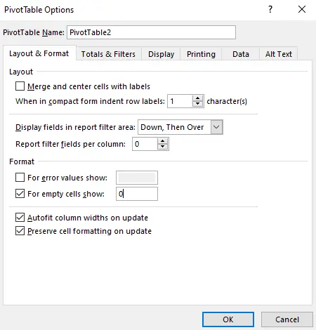
If the conditional formatting doesn’t work in the entire PivotTable, my first guess is that you might have empty cells. To deal with that, open PivotTable options and set zero for empty cells if that is logical.

If you want to delete or change PivotTable conditional formatting, you can do that as usual. Go to the Conditional Formatting tool in the Excel Home tab and choose Manage Rules at the end of the list.
There are other useful things that you can do with Excel PivotTable. For example, you can easily explore data distribution by creating a histogram or calculating a weighted average.