Get quarter in Excel from date – fast and easy

As usual in Excel, there is more than one way to get identical results, and the same happens if you try to get a quarter in Excel from date. Excel has multiple functions to do calculations with dates, but at this point, none of them are for quarter calculation.

The quarter in Excel form date is obtainable like this. I assume that your date is in cell A2.

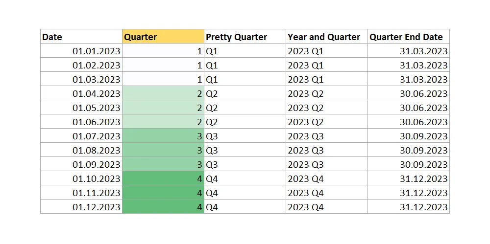
=INT(
(MONTH(A2) + 2) / 3
)

Function INT rounds a number down to the nearest integer. By knowing that it is necessary to add 2 to the month number. After dividing by 3 and rounding down, you will always get the corresponding quarter. Little play with numbers similar to ISO year calculation in Excel.

If you want, you can combine the result with “Q” or other text like this.

="Q" & INT(
(MONTH(A2) + 2) / 3
)

Here is how to combine year and quarter.

=YEAR(A2) & " Q" & INT(
(MONTH(A2) + 2) / 3
)

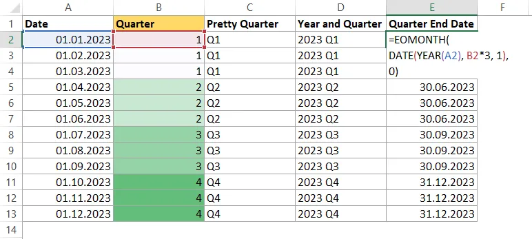
Excel formula for the quarter end date

If you want to know which date is at the end of the quarter and you have columns with the date and quarter or year and quarter, you can calculate that like this.

=EOMONTH(
DATE(YEAR(A2), B2*3, 1),
0)

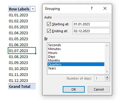
Quarter in Excel PivotTable

If you are summarizing your data with PivotTable, it is applicable to group dates in quarters. In that situation, no formulas are necessary.

Add date column to rows and columns, right-click on any of the dates and choose group. The next will be a window, as in the picture below, and you can choose how to group dates. You can select multiple grouping parameters.

Thank you for reading this post, and please look at other Excel-related posts in this blog.