How to use an image in a chart background in R

There are different ways how to use an image as the chart background in R. You can add that only in the panel background or plot background, or you can put the plot on top of the image.

Here is the dataset that I will use in a couple of examples.

require(dplyr)

cw <- chickwts %>%
  group_by(feed) %>%
  summarise('mean_weight' = round(mean(weight), digits = 0)) %>%
  arrange(desc(mean_weight)) %>%
  # mutate('feed' = forcats::fct_inorder(feed)) %>%
  mutate('feed' = factor(feed, levels = feed))

cw

## A tibble: 6 x 2
#  feed      mean_weight
#             
#1 sunflower         329
#2 casein            324
#3 meatmeal          277
#4 soybean           246
#5 linseed           219
#6 horsebean         160

Here is how it looks like a column chart. Here is a post from this blog about column or bar chart data labels, but I would like to change the background in different ways.

require(ggplot2)

cw %>%
  ggplot(aes(x = feed, y = mean_weight)) +
  geom_col(fill = "#6667AB",
           width = 0.5,
           alpha = 0.7) +
  labs(x = "feed", y = "mean weight, gm") +
  theme_minimal()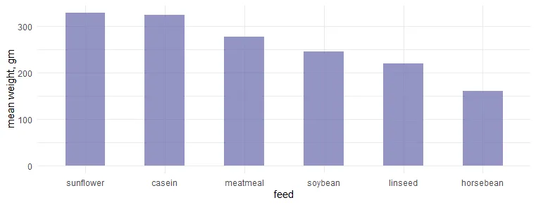

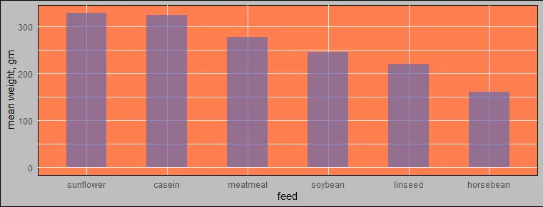
If you are struggling to understand the difference between the panel or plot background, then here is how it looks if there are modifications in the panel or plot background that can help to distinguish the differences between them.

cw %>%
  ggplot(aes(x = feed, y = mean_weight)) +
  geom_col(fill = "#6667AB",
           width = 0.5,
           alpha = 0.7) +
  labs(x = "feed", y = "mean weight, gm") +
  theme_minimal() +
  theme(
    panel.background = element_rect(fill = "coral")
    , plot.background = element_rect(fill = "grey")
  )

Prepare the image in R by adjusting opacity and other things

Here is the source of the image that I will use as the background, and here is how it looks.

require(magick)

img <- image_read("https://unsplash.com/photos/yEW23jxVsNI/download?ixid=MnwxMjA3fDB8MXxhbGx8fHx8fHx8fHwxNjY2ODc2MzAw&force=true&w=800")

## A tibble: 1 x 7
#  format width height colorspace matte filesize density
#                   
#1 JPEG     800    267 sRGB       FALSE        0 72x72  


img %>% image_scale("400")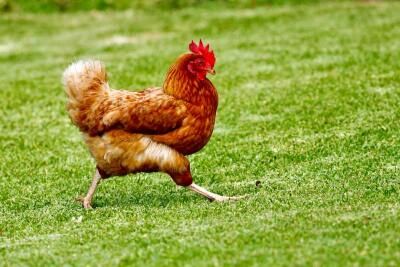

After reading images with package magick, it gives additional information about dimensions that I will use to resize the R column chart. Otherwise, with the function image_info you can read that later.

image_info(img)

For me, it was necessary to make some adjustments to incorporate the picture with the column chart. Luckily for me, there is package magick that is very useful to process images in R.

Before I was familiar with this package, I had no idea that it is possible to flip images horizontally, use blurry effects, or create faded colors in R. Here is the process of transformations and the result.

img2 <- img %>%
  image_flop() %>%
  image_blur(5, 5) %>%
  image_colorize(opacity = 70, color = "white")


image_append(c(img, img2)) %>% image_scale("800")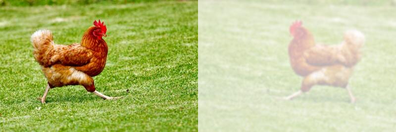

Here is a good intro about package magick and one additional one.

Add the image in the chart panel background in R ggplot2

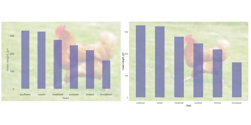
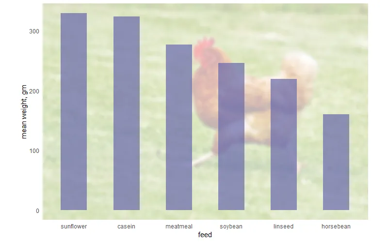
The first example is the image in the ggplot2 chart panel background by using annotation_custom and little help from the package grid. At the same time, I’m changing the chart aspect ratio to better match the image.

cw %>%
  ggplot(aes(x = feed, y = mean_weight)) +
  annotation_custom(grid::rasterGrob(img2
                                     , width = unit(1, "npc")
                                     , height = unit(1, "npc"))) +
  geom_col(fill = "#6667AB",
           width = 0.5,
           alpha = 0.7) +
  labs(x = "feed", y = "mean weight, gm") +
  theme_minimal() +
  theme(aspect.ratio = 533 / 800)


ggsave(
  "C:\\Users\\dc\\Downloads\\chicken_in_background.png",
  width = 800,
  height = 500,
  units = "px",
  dpi = 100,
  bg = "white"
)

Alternatively, you can use the annotation_raster like this.

cw %>%
  ggplot(aes(x = feed, y = mean_weight)) +
  annotation_raster(as.raster(img2), -Inf, Inf, -Inf, Inf) +
  geom_col(fill = "#6667AB",
           width = 0.5,
           alpha = 0.7) +
  labs(x = "feed", y = "mean weight, gm") +
  theme_minimal() +
  theme(aspect.ratio = 533 / 800)

There is also worth mentioning the package ggpubr that uses background_image to do the same as in previous examples.

require(ggpubr)

cw %>%
  ggplot(aes(x = feed, y = mean_weight)) +
  background_image(img2) +
  geom_col(fill = "#6667AB",
           width = 0.5,
           alpha = 0.7) +
  labs(x = "feed", y = "mean weight, gm") +
  theme_minimal() +
  theme(aspect.ratio = 533 / 800)

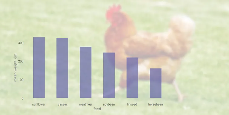
Add the image in the chart plot background in R ggplot2

Another option is to put the image in the ggplot2 plot background. To make the chart look better for that purpose, I made adjustments in the font size, color, etc.

p <- cw %>%
  ggplot(aes(x = feed, y = mean_weight)) +
  geom_col(fill = "#6667AB",
           width = 0.5,
           alpha = 0.7) +
  labs(x = "feed", y = "mean weight, gm") +
  theme_minimal(base_size = 16) +
  theme(
     panel.grid.major = element_blank()
    ,panel.grid.minor = element_blank()
    ,axis.title.x = element_text(colour = "grey50", size = 14)
    ,axis.title.y = element_text(colour = "grey50", size = 14)
  )

p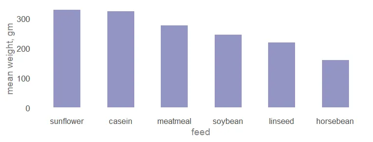

With the package cowplot, it is possible to put the chart on top of the image and create necessary adjustments.

require(cowplot)

ggdraw() +
  draw_image(img2, scale = 1.35) +
  draw_plot(p, x = -0.1, y = -0.13, scale = 0.7)

It is worth mentioning the package ggimage that can help similarly.

If you like to have an interactive chart, then here is how to use background images in the plotly.

Thank you for reading this and please look at the other data visualization from this blog.