How to add legend title in Excel chart

At this moment, there is no default and easy way how to add a legend title in an Excel chart. The good news is that you can create that on your own. Here is a simple instruction on how to add legend titles in Excel efficiently.

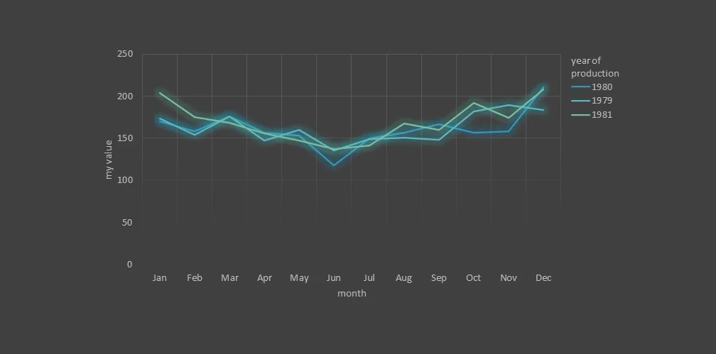
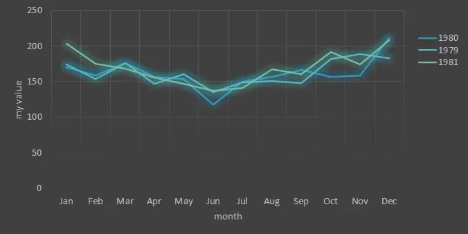
Here is my Excel chart without a legend title. How to add a legend, and create basic formatting you can find here.

If you want to know how to create this Excel chart with a glow effect, take a look at this post.

Add legend title in Excel chart

1. Select an Excel chart to add a text box. This is important to bound chart and textbox together. Otherwise, the Excel chart and text box move separately.
2. Go to the Insert tab, and on the right side will be a text box. Selec and draw it over the place where you want it in the chart.
3. If you want the text in the same formatting as in the legend, try format painter. Select legend, click on format painter, and then on the text box.

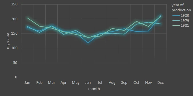
As a result, here is my Excel chart with added legend title. Make sure that your chart is at the right size because the text box is not changing size or position as perfectly as other default chart elements.

Format painter is one of the best time savers in Excel. Here is how to copy formatting from one Excel chart and apply it to another.

If you are resizing some of the Excel chart elements, it might cause problems. It looks like the inability to resize elements automatically when you change the whole size. Here is how to reset the Excel chart layout.

You might like other Excel-related posts in this blog. For example, how to use PivotTable to create a histogram.