4 ways how to create a gradient word cloud in R

If you have a gradient word cloud in R, then besides the size of each word representing results, an additional indicator is also the color. Here are 4 ways how to create that kind of word cloud in R using packages like ggplot2, quanteda, wordcloud, and wordcloud2.

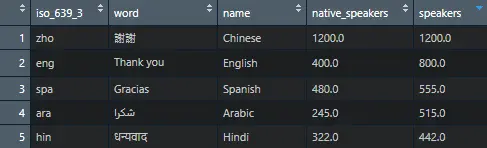
To get the necessary data and functionality for ggplot2, I will use the ggwordcloud package. There is a data set called thankyou_words that contains useful data. Speakers are the number of speakers in millions and represent a quantity parameter for each word.

require(ggwordcloud)

tw <- thankyou_words_small

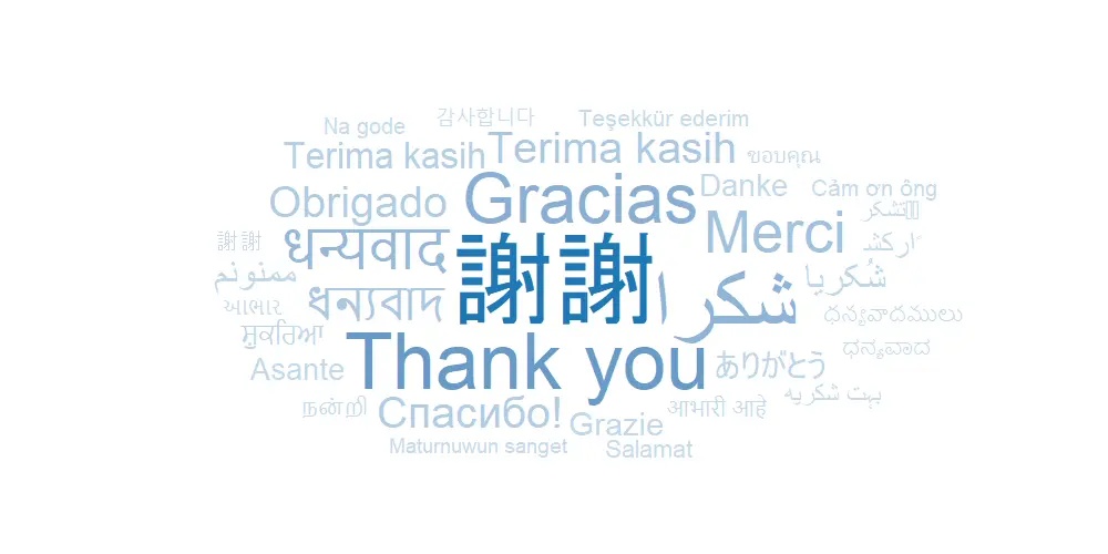
Create a gradient word cloud in R with the ggplot2 package

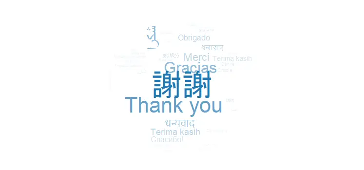
Package ggplot2 comes with the function scale_color_gradient which is useful to create a gradient word cloud in R. Take a look at the post about gradient line chart in R.

Word cloud with ggplot2 can be obtained thanks to ggwordcloud text geom. The ggwordcloud comes with a lot of arguments that you can change. For example, eccentricity makes it taller or wider.

require(ggplot2)


set.seed(42)

ggplot(data = tw, aes(label = word, size = speakers, color = speakers))+
  geom_text_wordcloud_area(area_corr_power = 1, eccentricity = 1)+
  scale_size_area(max_size = 25) +
  scale_color_gradient(low = "#C7DDEC", high = "#1F78B4") +
  theme_minimal()

There are multiple ways how to deal with colors in ggplot2. Here is a document that contains all color names that can be used straight forward. I like my cloud to be blue, and I picked a few colors by hex color codes.

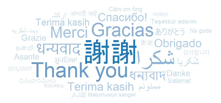
Create a gradient word cloud in R with the quanteda package

For me, the word cloud with quanteda is interesting because it can nicely overlap words in the word cloud. You can create that with the function textplot_wordcloud.

The main problem is that data for the word cloud should be in the document term matrix (DFM in quanteda). First of all, I will transform my R data frame to DFM with help of the cast_dfm function from the tidytext. Here you can learn more about the process.

require(tidytext)
require(dplyr)

tw_trans <- tw %>% 
  select('term' = word, 'count' = speakers) %>% 
  mutate('document' = 1)

tw_trans <- tw_trans %>%
  cast_dfm(document, term, count)

After the data frame is transformed to a document feature matrix, you can use that in textplot_wordcloud from quanteda. The gradient is created by generating hex color codes.

require(quanteda)

col <- sapply(seq(0.1, 1, 0.1), function(x) adjustcolor("#1F78B4", x))

textplot_wordcloud(
  tw_trans,
  adjust = 2,
  color = col
)

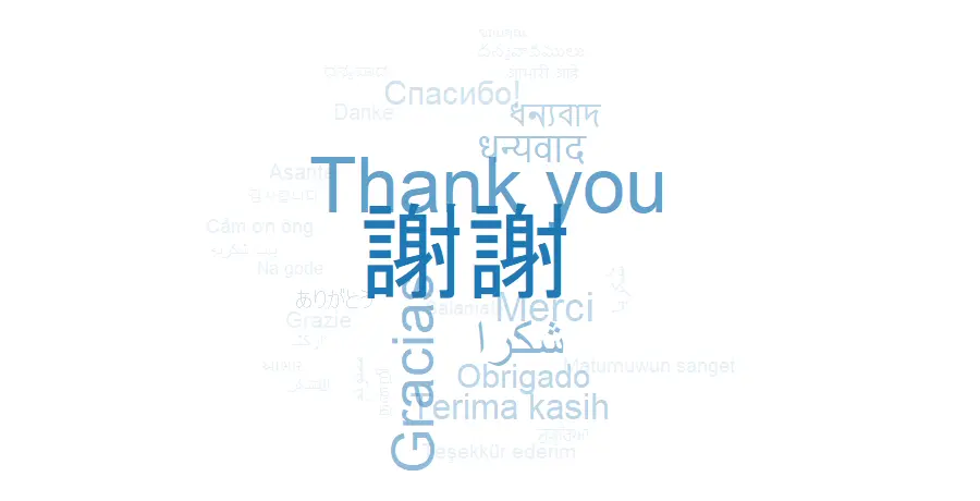
packages wordcloud and wordcloud2

There are another two options for gradient word clouds in R. By using the worcloud2 package, you can get that interactive, and it is an obvious advantage.

For the wordcloud function, I generated hex color codes the same way as in the example with quanteda.

library(wordcloud)

col <- sapply(seq(0.1, 1, 0.1), function(x) adjustcolor("#1F78B4", x))

wordcloud(
  tw$word,
  tw$speakers,
  scale = c(4, 0.25),
  random.order = FALSE,
  random.color = FALSE,
  colors = col
)

If the word cloud cuts off text closer to borders, you should play around with the scale argument.

With the wordcloud2, it is a little bit trickier to get the necessary color gradient. Depending amount of words, there should be generated hex color codes. After experimenting with that, I decided that there should be one hex color code for every 4 words.

require(wordcloud2)

n <- ceiling(nrow(tw)/4)

col <-
  sapply(sapply(seq(
    from = 1, to = 0.25, by = -0.25
  ), rep, n), function(x)
    adjustcolor("#1F78B4", x))

wc2 <- tw %>% select(word, 'freq' = speakers)

wordcloud2(wc2, color = col)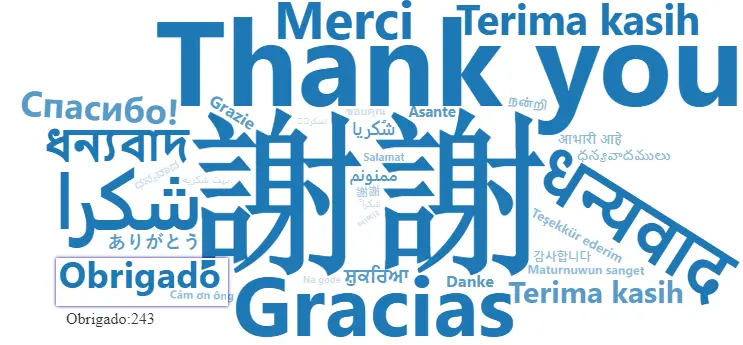

This is one of my favorite results of all the gradient word clouds in R. I published it as a picture, but you can get interactive HTML visualization.

Take a look at these posts to learn more about generating hex color codes and repeated sequences in R.